
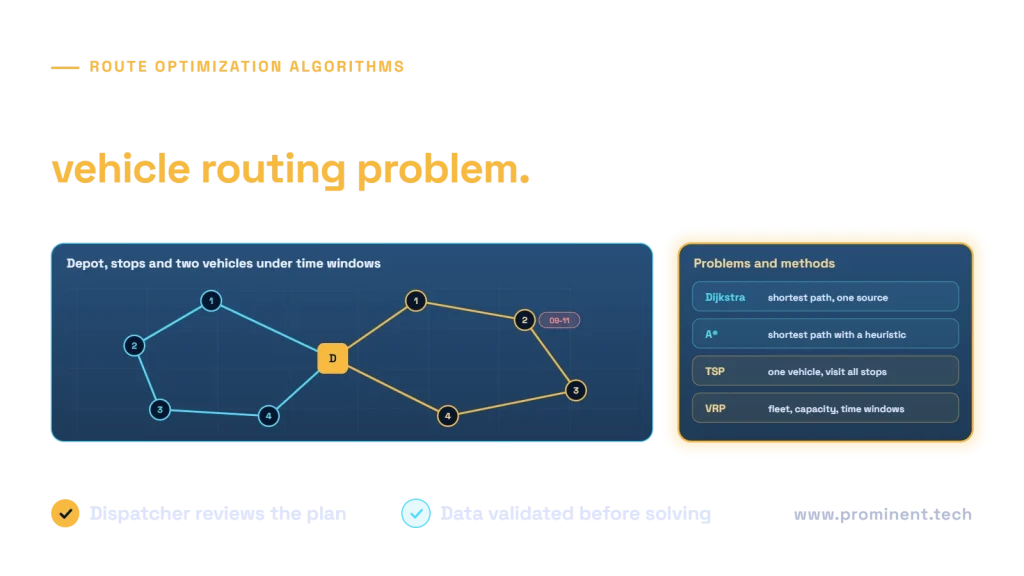
Dijkstra and A* find paths through a graph; TSP and VRP describe visit-order and fleet-planning problems. A delivery operation normally needs more than a shortest path: it must assign stops to vehicles while respecting capacity, time windows, service times and operating rules. AI can improve travel-time estimates or demand predictions, but a routing solver must still produce a feasible plan. Measure useful routes against the same constraints and workload.
Key takeaways
- Distinguish the road-network path from the fleet’s stop sequence.
- Validate coordinates, service times, capacity units and time windows before solving.
- A* depends on a suitable heuristic; Dijkstra requires nonnegative weights.
- VRP heuristics can find useful solutions without proving a global optimum.
- AI-predicted costs do not remove legal or operational constraints.
- Dispatchers need an exception and override process when conditions change.
How route optimization works
Begin with the business objective: minimize travel, meet service windows, control overtime or balance workload. Collect validated stops, vehicle availability, depots and constraints. Geocode addresses and review ambiguous locations. Obtain a travel-time or distance matrix appropriate to the vehicle and time context. Formulate the fleet problem, solve within a time budget, verify feasibility and let the dispatcher approve the plan. Monitor actual execution and investigate differences.
A straight-line distance matrix may be useful for teaching but is not a road-routing model. Roads can be one-way, have access restrictions or change with traffic. Travel time can be asymmetric. A service visit also consumes time at the customer; omitting unloading or inspection duration makes an apparently feasible schedule unrealistic. Keep matrix units and service-duration units consistent.
Dijkstra’s algorithm explained
Dijkstra repeatedly expands the unsettled node with the lowest known distance from the source. With nonnegative edge weights, settling a node establishes its shortest-path distance under the algorithm’s assumptions. It can compute paths to many destinations from one source. With adjacency lists and a binary heap, a common complexity bound is O((V + E) log V); a simple array implementation has different behavior.
distance[source] = 0
priority_queue.push((0, source))
while priority_queue is not empty:
    cost, node = pop_smallest()
    if cost != distance[node]: continue  # stale entry
    for neighbor, nonnegative_weight in edges[node]:
        candidate = cost + nonnegative_weight
        if candidate < distance[neighbor]:
            distance[neighbor] = candidate
            predecessor[neighbor] = node
            priority_queue.push((candidate, neighbor))
The graph must represent the desired cost. Minimizing distance is different from minimizing time or toll cost. Negative edge weights invalidate the standard Dijkstra guarantee. Restrictions should remove or appropriately constrain prohibited movements; assigning a small penalty to an illegal route does not make it legal. Store the path’s predecessor chain if the application needs the actual route rather than only the cost.
A* search explained
A* orders candidates by f(n) = g(n) + h(n): known cost from the start plus an estimate of remaining cost. An admissible heuristic does not overestimate the remaining optimal cost. Graph-search implementations also need appropriate handling of improved paths; consistency is a useful condition for implementations that do not reopen settled nodes. Setting h to zero reduces A* to Dijkstra-style search. A poorly chosen heuristic can remove the shortest-path guarantee.
For geographic distance, an appropriate lower bound may guide search. For travel time, distance divided by an unrealistic speed is not automatically safe: the units and bound must be justified. A* can explore fewer nodes with a useful heuristic, but it is not universally faster. The NetworkX A* reference explicitly warns that an overestimating heuristic may return a non-shortest path.

TSP and VRP are problems, not individual algorithms
| Term | Question | Typical constraint |
|---|---|---|
| Shortest path | How should one origin reach a destination? | Road-network permissions and edge costs |
| TSP | In what order should one tour visit locations? | Visit each required location |
| CVRP | How should a fleet serve demand? | Vehicle capacity |
| VRPTW | How should a fleet meet service windows? | Arrival times, waiting and service duration |
| Pickup and delivery | How should paired tasks be scheduled? | Precedence and same-vehicle requirements |
| Dynamic routing | How should a changing plan be updated? | New requests, traffic and disruption |
VRP variants can combine capacity, working hours, skills, vehicle types, breaks and depot rules. These constraints can conflict, leaving no feasible solution. The application must distinguish infeasibility from solver timeout and from a valid solution whose quality is not proven optimal. Silently dropping a customer is not acceptable unless optional service and its penalty are an explicit business rule, visibly reported to the dispatcher.

Which algorithms solve vehicle routing problems?
Exact methods such as mixed-integer optimization and branch-and-bound can prove optimality for suitable formulations and manageable instances. Constraint programming and specialized routing solvers can express many operational constraints. Construction heuristics build an initial plan; local search improves it through moves such as relocating or swapping stops. Metaheuristics help explore beyond local improvements. The practical choice depends on problem size, constraints, response-time budget and the value of proving optimality.
A ten-second planning deadline may favor a feasible, explainable solution over an exact proof that takes much longer. Conversely, an offline strategic decision may justify more computation. Report the search configuration, time limit, feasibility and objective. Do not call every solver result “the optimal route.” If a bound or optimality gap is unavailable, say so.
How AI can improve routing inputs and decisions
| AI contribution | Useful output | Boundary |
|---|---|---|
| ETA prediction | Travel-time estimates by context | Validate against future conditions and road restrictions |
| Demand forecasting | Expected stop or shipment demand | Uncertainty affects capacity planning |
| Service-time prediction | Expected duration at a stop | Include variance and accessibility needs |
| Disruption detection | Potential incident or delay | Confirm operational significance |
| Dispatch assistance | Ranked scenarios or explanations | Solver feasibility and dispatcher authority remain separate |
A model trained on historical routes may encode driver behavior, data gaps or past service inequities. Evaluate the prediction where it will be used and monitor drift. A generated explanation should reflect actual constraints and solver output, not invent a reason for a sequence. Reinforcement-learning methods can be researched, but production adoption requires evidence on feasibility, robustness and comparison with strong conventional solvers.
Enterprise routing architecture

Use stable order and stop identifiers, versioned constraints and a planning run ID. Save the matrix timestamp, solver configuration, approved plan and overrides. Dispatch should receive an immutable approved version; changes require a new version with a visible difference. If an external map API fails, use a defined fallback or stop planning rather than silently substituting unsuitable costs.
Protect address and driver data through purpose-limited access and retention. Avoid placing unnecessary personal information into solver logs. Integrate order status and proof-of-service through explicit APIs with idempotent updates. A route completion event should reconcile with the order system so repeated messages do not create duplicate business effects.
Python and Google OR-Tools: a small constrained example
Download the supporting source and diagrams (.zip)
Local synthetic run: all four customers were visited exactly once, each vehicle load was four units within capacity, and the returned time-window constraints passed independent checks. This is a feasible result, not proof of global optimality.
The downloadable route-example.py models two vehicles, four synthetic customers, integer demand, capacity and time windows. Travel and service times are in minutes. It uses a fixed synthetic matrix—not live traffic—and reports the selected routes, load and time values. The script independently checks that every required customer appears exactly once and that capacities, time windows and route transitions are feasible. Its result is a teaching example, not a road-network benchmark.
# Core callback contract; see the complete downloadable script.
def travel_with_service(from_index, to_index):
    i = manager.IndexToNode(from_index)
    j = manager.IndexToNode(to_index)
    return time_matrix[i][j] + service_minutes[i]

# Use the callback for a Time dimension with allowed waiting.
# Apply customer windows to CumulVar(manager.NodeToIndex(customer)).
# Apply depot windows to each vehicle's Start and End indices.
# Add a separate demand/capacity dimension using consistent units.
# No solution must be handled explicitly; never invent a route.
Routing indices are not always the same as node indices; use the index manager. Service time is attached to departure from the visited node in this formulation, so cumulative time represents arrival. Waiting is allowed within the configured slack. Keep this convention consistent when checking time windows. The OR-Tools VRPTW guide explains the underlying routing and time-dimension concepts; production constraints must be added explicitly.
Platforms and APIs are not interchangeable
| Option | Provides | Evaluate |
|---|---|---|
| Google OR-Tools | A solver library operated by your application | Modeling, runtime and support ownership |
| Google Maps routing or optimization services | Managed geographic or optimization capabilities depending on API | Terms, limits, supported constraints and regional pricing |
| Azure Maps | Geospatial search, routing and matrix capabilities | Selected API, vehicle options, geography and quotas |
| Specialized planning platform | Workflow, dispatch and optimization features | Constraint fit, integrations and exportability |
| Custom hybrid | Selected map data plus a controlled solver | End-to-end operational ownership |
The Azure Maps overview describes several routing capabilities. Verify the exact endpoint, region, vehicle restrictions and commercial terms before selecting it. A point-to-point route API is not necessarily a fleet optimization API. Map coverage and specialized commercial-vehicle support should be tested in the operating geography, not assumed from a product overview.
Industry applications and their constraints
| Industry | Planning task | Constraint that changes the model |
|---|---|---|
| Delivery and retail | Multi-stop distribution | Capacity, time windows and failed-delivery rules |
| Field services | Technician visits | Skills, parts and appointment durations |
| Healthcare logistics | Transport of supplies or samples | Handling, timing and approved protocols |
| Manufacturing | Inbound and plant logistics | Dock availability and production schedules |
| Waste services | Collection routes | Service coverage and vehicle limits |
| Utilities | Inspection and repair visits | Priority, access and safety procedures |
Measure performance and ROI fairly
Compare plans with the same required stops, constraints and operating period. Report unserved stops, late arrivals, route duration, total distance, overtime and workload distribution. Include solver runtime, dispatch review and plan stability. A shorter plan that violates a customer window or vehicle capacity is not a better plan. Use actual execution data to evaluate travel estimates and explain changes caused by traffic or customer availability.
Hypothetical monthly example: a defensible 8,000-unit reduction in travel expense plus 4,000 of distinct overtime reduction, less 5,000 of API, support and operating cost, gives 7,000 units net value. With 42,000 initial integration cost, simple payback is six months under those assumptions. This is illustrative arithmetic. Do not count fuel already included in travel expense a second time or use predicted distance reduction as realized savings before execution evidence exists.
Implementation roadmap and production checklist
- Define objectives, legal constraints and the dispatcher’s authority.
- Validate addresses, vehicle data, service times and units.
- Build a baseline plan from the current operating process.
- Prototype a small feasible model and inspect exceptions.
- Backtest comparable days and stress unusual workloads.
- Pilot with dispatchers and preserve manual recovery.
- Integrate approved plans, status updates and monitoring.
- Version releases and evaluate actual operational outcomes.
Before release, test impossible windows, unavailable vehicles, disconnected customers, duplicate orders, API outages and delayed updates. Verify privacy controls, accessibility, timezone conventions and driver communication. Define how accepted commitments are preserved during replanning and who can authorize a changed route. Monitor plan freshness so an outdated route is never displayed as current.

Frequently asked questions
What is the difference between Dijkstra and A*?
Dijkstra expands by known distance from the source, while A* adds a heuristic estimate of remaining cost. With suitable assumptions both can find shortest paths. An unsuitable heuristic can invalidate A*’s guarantee. Neither algorithm alone solves the full multi-vehicle assignment problem.
Are TSP and VRP algorithms?
No. They are problem definitions. TSP concerns a tour through locations; VRP adds fleet assignment and operational constraints. Many exact methods, heuristics and specialized solvers can address variants of these problems.
Can Dijkstra use negative weights?
The standard algorithm requires nonnegative edge weights. Negative weights invalidate its usual correctness reasoning. In road planning, also check that the chosen weights represent the intended distance, time or cost objective and that prohibited movements are handled appropriately.
Does A* always run faster?
No. Its practical benefit depends on the heuristic, graph and implementation. A useful admissible heuristic can reduce exploration; a weak one may offer little benefit. Report measured behavior for the actual problem instead of claiming universal speed superiority.
Does OR-Tools guarantee the best possible route?
Not for every configuration or time-limited search. It can find useful feasible solutions to routing problems, but a selected heuristic result may not include proof of global optimality. Record the search limits, constraints and solution status.
Can AI replace the routing solver?
AI can improve ETA, demand or service-time predictions and support dispatch decisions. A production plan still needs constraint validation. A fluent explanation or predicted route sequence is not proof that capacity, working hours and customer windows are satisfied.
What data is required?
Validated locations, vehicle availability, capacities, customer demand, service durations, time windows and suitable travel costs are common inputs. The actual model may need skills, breaks, depots and legal restrictions. Units and time conventions must be explicit.
How does real-time traffic affect routing?
It can change travel estimates and make an existing plan less suitable. Replanning should preserve accepted commitments, report changed assignments and avoid unnecessary instability. Verify the map provider’s supported traffic behavior and the freshness of the data.
What happens when no feasible plan exists?
Report the status and conflicting requirements rather than inventing a route. A dispatcher may add capacity, renegotiate a window or explicitly approve an optional stop policy. Keep such business decisions visible and separate from silent solver adjustments.
How should route savings be measured?
Compare equivalent workloads and constraints, then verify actual distance, expense, overtime and service outcomes. Include review and platform costs. Do not count the same cost twice or treat an infeasible shorter route as an improvement.
Can a routing API handle every truck restriction?
Do not assume so. Validate the selected API, endpoint, geography and vehicle parameters against the operation’s requirements. Map coverage and restrictions vary, and the fleet remains responsible for an appropriate operating and safety process.
Where should an enterprise start?
Start with a bounded planning area and reliable data. Reproduce current constraints, establish a baseline and inspect a small solver result with dispatchers. A feasible, reviewable pilot is more useful than a large model with incomplete operating rules.
Technical references
Technical source review: 1 November 2026. Illustrative architectures, assumptions and examples are not client implementations or measured production results. Deployment-specific verification is required.