
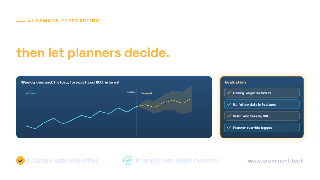
AI demand forecasting uses historical demand and relevant information available at the planning cutoff to estimate future demand. Statistical and machine-learning models can support inventory, staffing and capacity decisions, but no model removes uncertainty. Start with a seasonal-naive baseline, evaluate at the actual business horizon and convert forecasts into decisions through lead-time, service-level and operating constraints. Generative AI is not a substitute for a validated numerical forecasting model.
A retailer ordering inventory for next month has a different problem from a manufacturer scheduling next week or a utility planning tomorrow. The target, time granularity, available inputs and cost of errors all change. A useful project therefore begins with the decision and its timing, rather than choosing the most complex model. This guide explains the data, models and evaluation methods needed to make that decision measurable.
Key takeaways
- Observed sales can understate demand during stockouts.
- Only use information available when the forecast would have been issued.
- Compare models against a seasonal baseline at the same horizon.
- Measure error by segment and business consequence, not only a pooled score.
- Use uncertainty and operational constraints in the planning decision.
- Keep planner overrides traceable and evaluate whether they help.
What exactly should the system forecast?
Specify the item, location, time bucket, horizon and target definition. Sales, orders, fulfilled units and unconstrained demand are not interchangeable. Returns, cancellations, substitutions and promotions need explicit treatment. An apparent increase in accuracy can come from changing the target rather than improving the planning decision. Record how demand is measured and which unavailable observations are excluded or estimated.
Define the forecast issue time and data cutoff. A weekly four-week-ahead forecast cannot use tomorrow’s actual sales or next month’s observed weather. It can use a promotion schedule already approved at the cutoff, or a weather forecast that was available then. Store vintage forecasts for external variables where possible. Using realized future covariates during backtesting produces an evaluation the production system cannot reproduce.
| Data source | Useful information | Potential trap |
|---|---|---|
| ERP and orders | Orders, cancellations and lead times | Changes after the historical cutoff |
| POS and inventory | Sales, availability and stockouts | Treating censored sales as full demand |
| Pricing and promotions | Known plans and historical events | Using final plans not known at issue time |
| Calendar | Holidays, weekdays and seasonality | Different local calendars |
| Weather and external data | Available forecasts or past observations | Future realized values leaking into features |
| Product metadata | Category, lifecycle and substitutions | Obsolete mappings and cold-start items |
Forecasting model comparison
| Model | Useful starting point | Main limitation |
|---|---|---|
| Seasonal naive | Repeat comparable prior season | Cannot explain new structural changes |
| Moving average or ETS | Stable level, trend or seasonality | Abrupt changes and sparse histories |
| ARIMA or SARIMA | Autocorrelation and defined seasonal structure | Model assumptions and many separate series |
| Prophet | Trend and calendar-oriented baseline | Not an automatic winner for every series |
| Random forest | Nonlinear tabular features | Extrapolation and horizon construction |
| Gradient boosting | Lag, calendar and known driver features | Leakage and iterative forecast design |
| LSTM or GRU | Temporal sequences with sufficient data | Training burden and data requirements |
| DeepAR or TFT | Global probabilistic or multi-series modeling | Complexity, tuning and operating cost |
| Croston-style methods | Intermittent nonnegative demand | Assumptions and changing occurrence patterns |
A local model learns each series separately; a global model learns across related series using identifiers and attributes. Global models can share information but may underperform for poorly represented groups. A cold-start item may need category history, analogous products or a planning rule because its own lag features do not exist. Intermittent demand requires attention to both occurrence and size, not simply a larger neural network.
Hierarchical forecasts should be reconciled when decisions require consistent totals across product, region and organization. Evaluate the levels that matter to planners. Good aggregate accuracy can hide serious item-location errors. Conversely, an item-level model may produce inconsistent regional totals unless reconciliation is part of the process.
An architecture for forecasts and reviewed decisions

Use a versioned data snapshot and feature contract for each training run. Save model versions, forecast issue times, horizons and prediction intervals. A forecast table should identify the model and target period explicitly; overwriting yesterday’s predictions destroys evaluation evidence. Separate the numerical forecast from narrative explanations, and do not let a generated narrative invent a causal explanation unsupported by the inputs.
The planning layer combines forecast distributions with stock, lead times, capacity and business policy. An inventory decision may need a service-level or cost trade-off; a staffing decision must respect skills and employment constraints. A planner can override the forecast, but the system should preserve the original, reason, author and date so the value of overrides can be measured.
Accuracy metrics: formulas and interpretation
| Metric | Definition | Use and caution |
|---|---|---|
| MAE | Mean of absolute errors | Readable in original units; scale-dependent |
| RMSE | Square root of mean squared errors | Penalizes large errors more strongly |
| MAPE | Mean absolute percentage error | Undefined at zero actual demand; unstable near zero |
| WAPE | Sum absolute error / sum actual demand | Volume-weighted aggregate; denominator can be zero |
| MASE | MAE / training naive-error scale | Use the correct seasonal lag and training-only scale |
| RMSSE | Root mean squared error / training squared-difference scale | State the exact scaling convention |
| Bias | Mean forecast minus actual | Positive means overforecast under this convention |
| Pinball loss | Asymmetric error for a chosen quantile | Useful when under- and overforecast costs differ |
A synthetic four-period example has actual demand [100, 120, 80, 100] and forecast [90, 130, 100, 80]. Absolute errors are [10, 10, 20, 20]. MAE is 15 units; RMSE is √250, approximately 15.81; WAPE is 60 / 400 = 15%; MAPE is approximately 15.83%. Mean forecast-minus-actual bias is zero. Zero bias therefore does not mean zero error: over- and underforecasts can cancel. If the training seasonal-naive absolute-error scale is 12 units, MASE is 1.25.
For a median forecast, pinball loss uses the 0.5 quantile; for inventory planning, another quantile may be more appropriate after accounting for the actual cost structure. A higher quantile is not inherently more accurate—it encodes a different decision trade-off. Evaluate interval coverage together with interval width. Extremely wide intervals can achieve high coverage without being useful.
The forecasting principles in Forecasting: Principles and Practice support a careful distinction between fitted residuals and genuine forecast errors. A model that closely fits history may still forecast poorly. Report a backtest that reproduces the intended issue dates and horizons rather than quoting training-set fit.
Backtesting without future-data leakage
Use rolling-origin evaluation: fit with data up to a cutoff, forecast the required future periods, advance the cutoff and repeat. Keep the final holdout untouched until model selection is complete. Report performance by horizon because one-step results do not establish four-week performance. Fit preprocessing and feature selection within the training window. Avoid random row splits on lagged time-series observations.

The scikit-learn lagged-feature example illustrates why time-aware evaluation matters. Production design also requires multi-step availability checks: lag 1 for tomorrow is known, but lag 1 for the fourth future day is not known at the original issue time. Use direct horizon models, a carefully evaluated recursive process or another explicit strategy rather than silently supplying future actuals.
A small, executable forecasting example
Download the supporting source and diagrams (.zip)
Local synthetic run: candidate MAE 4.18 units versus seasonal-naive MAE 4.10. The candidate did not outperform the baseline; these values are specific to this educational dataset.
The downloadable Python example generates synthetic daily demand, creates a one-step lag plus known calendar features, splits chronologically and compares a simple fitted model with a same-weekday baseline. It uses only the Python standard library. It is an educational one-step evaluation, not a production demand model or a benchmark. Each later test prediction assumes the preceding actual observation has arrived; it must not be described as a fixed-origin multi-week forecast.
# One-step evaluation contract:
# 1. At day t, yesterday's actual is available.
# 2. Weekday is known; future realized demand is not.
# 3. Fit coefficients on training rows only.
# 4. Compare with demand from t-7 on identical test dates.
# See forecast-example.py for the executable synthetic demonstration.
# A multi-step forecast requires a different availability design.
Ten implementation steps and acceptance checks
| Step | Deliverable | Acceptance question |
|---|---|---|
| 1. Define decision | Target, horizon and cost of error | Can the planner act at that horizon? |
| 2. Audit data | Sources, cutoffs and stockout handling | Are past information vintages reproducible? |
| 3. Establish baseline | Seasonal-naive and current-plan scores | Are dates and denominators comparable? |
| 4. Segment series | Volume, intermittency and lifecycle groups | Are important groups represented? |
| 5. Engineer features | Past-only lags and known covariates | Would each feature exist at issue time? |
| 6. Compare models | Rolling-origin evidence | Does complexity improve useful measures? |
| 7. Test decisions | Inventory or capacity simulation | Are constraints and cost assumptions realistic? |
| 8. Pilot with planners | Reviewed forecasts and overrides | Can users inspect and challenge outputs? |
| 9. Operationalize | Versioned pipeline and fallback | Can forecasts be reproduced and recovered? |
| 10. Monitor | Error, drift and decision outcomes | Who investigates deterioration? |
Five industry applications
| Industry | Planning decision | Special consideration |
|---|---|---|
| Retail | Replenishment by item and location | Stockouts, promotions and substitutions |
| Manufacturing | Production and material planning | Lead times and capacity constraints |
| Logistics | Capacity and workforce allocation | Network effects and event demand |
| Healthcare operations | Administrative demand and staffing support | Safety, skills and access constraints |
| Energy and utilities | Load-related operational planning | Weather forecast vintages and local conditions |
These are illustrative planning contexts. The horizon, granularity and governance should reflect the actual organization. A forecasting component should not automatically change clinical staffing, contractual allocations or other consequential decisions without the relevant review and operating authority.
Twelve challenges that often matter more than model complexity
| Challenge | Response |
|---|---|
| Stockout-censored sales | Model availability and assess unmet demand explicitly |
| New products | Use analogues, metadata and controlled rules |
| Sparse demand | Evaluate intermittent-demand methods |
| Promotions | Use plans known at issue time |
| Structural breaks | Monitor and reassess the operating regime |
| Hierarchical inconsistency | Reconcile where decisions require consistent totals |
| Missing observations | Distinguish missing, closed and zero-demand periods |
| Returns and cancellations | Define the target and adjustment policy |
| Changing product identifiers | Maintain effective-dated mappings |
| Planner overrides | Preserve reasons and measure forecast value added |
| Unreliable external data | Track provider availability and vintages |
| Operational failure | Fallback forecast and visible freshness status |
Build, buy or combine—and estimate total cost
A planning product can provide workflow, integration and support that a standalone model does not. A custom model can suit a distinctive target or operating constraint, but it requires lifecycle ownership. A hybrid approach may preserve the planning system while introducing an evaluated forecasting component. Compare the ability to export forecasts, inspect assumptions, handle permissions and recover from failure—not only a vendor’s headline accuracy claim.
Cost includes data integration, quality work, evaluation, model execution, planning integration, monitoring and staff review. Hypothetical annual calculation: 180,000 currency units of separately justified inventory-related value plus 40,000 of distinct planning capacity, minus 100,000 recurring cost, gives 120,000 annual net value. With 240,000 initial cost, simple payback is two years under those assumptions. This is not a project quote or a promise of inventory reduction. Avoid counting reduced stock value as recurring profit without an appropriate financial treatment.
Evaluate service levels, stockouts, waste and working capital alongside forecast error. Lower average error does not automatically reduce costs if the relevant high-cost items worsen. Use realistic lead times and ordering constraints in the decision simulation. Pilot on a bounded segment and compare like-for-like periods before extending the scope.
Frequently asked questions
What is AI demand forecasting?
It estimates future demand from historical data and relevant information available at the planning cutoff. Machine learning is one possible method alongside statistical baselines. The forecast supports a decision; inventory, staffing and capacity constraints still need an explicit planning process.
Is generative AI a forecasting model?
A language model can help explain approved results or assist an analyst, but fluent text is not evidence of numerical forecast validity. Use a tested numerical method for the target and horizon. Check any generated explanation against the actual model inputs and evidence.
Which model is most accurate?
There is no universal winner. Compare seasonal naive, statistical and machine-learning candidates on the same rolling-origin tests. Data volume, intermittency, promotions and horizon affect results. Choose additional complexity only when it improves meaningful measures on independent evaluation data.
Why can sales differ from demand?
Sales may be limited by stock availability, capacity, substitutions or closed periods. A zero sale during a stockout does not necessarily mean zero customer demand. Record availability and define how constrained observations are treated before fitting or evaluating the model.
Should we use MAPE?
Use it carefully. MAPE is undefined when actual demand is zero and unstable near zero. MAE, WAPE, MASE, RMSSE or quantile-based measures may be more suitable depending on the decision. Report denominator conventions and segment results rather than relying on one score.
What is rolling-origin validation?
The model is trained up to a historical cutoff and predicts a specified future horizon, then the cutoff advances and evaluation repeats. It approximates real forecast issuance more closely than random row splitting. Features and preprocessing must use only information available at each cutoff.
How are new products forecast?
Use relevant product attributes, comparable items, category patterns and transparent planning rules when history is absent. Evaluate cold-start performance separately. A model trained on mature products may not generalize reliably to a new launch or a materially different product.
How should planner overrides be handled?
Preserve the original forecast, override, reason and timestamp. Evaluate whether overrides improve outcomes for comparable cases and horizons. Do not overwrite the model forecast, because doing so removes the evidence needed to measure both model and human contribution.
How much history is required?
It depends on seasonality, granularity, related series and the decision horizon. More data is not automatically better if business conditions have changed. Audit coverage and quality, establish a baseline and evaluate whether additional history helps the target groups.
When should a forecast model be retrained?
Use a schedule and monitoring policy appropriate to the planning process, with investigation of drift, errors and data changes. Evaluate new models before promotion. Retraining cannot fix a broken source feed, incorrect stockout treatment or a changed business target.
Technical references
Technical source review: 1 November 2026. Illustrative architectures, assumptions and examples are not client implementations or measured production results. Deployment-specific verification is required.